Appendix
Methodology for measuring and visualizing performance metrics
An overview of performance metrics used in HPC, and how to correctly visualize them.
Excellent resources from Torsten Hoefler (Gordon Bell Prize winner) on Scientific Benchmarking of Parallel Computing Systems:
Scalability
In the most general sense, scalability (or scaling) is defined as "the ability to handle more work as the amount of computing resources grows". For software, scalability is sometimes referred to as parallelization efficiency — the ratio between the actual speedup and the ideal speedup obtained when using a certain number of processors. The speedup in parallel computing can be straightforwardly defined as:
Where \(t_1\) is the computational time for running the software with one core (i.e. sequentially), and \(t_N\) is the computational time running the same software with N cores or processors. Ideally, we want software to have a linear speedup that is equal to the number of processors (i.e. \(Speedup = N\)). Unfortunately, this is a very challenging goal for real world applications to attain (see Amdhal's Law).
Scalability testing measures the ability of an application to perform well or better with varying problem sizes and numbers of processors. It does not test the applications general funcionality or correctness.
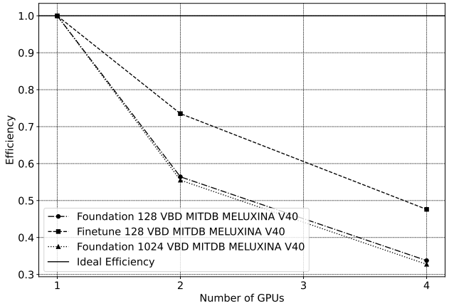
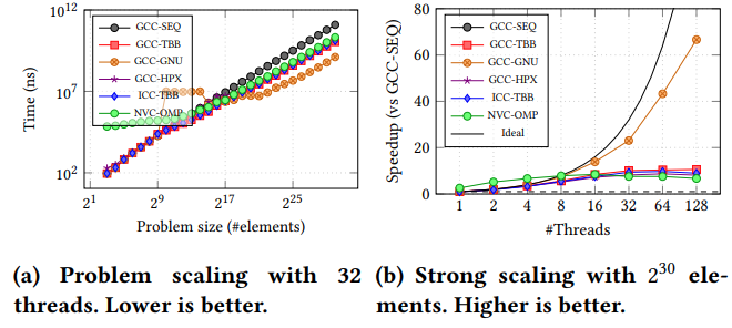
Strong scaling
In case of strong scaling, the number of processors is increased while the problem size remains constant. This results in a reduced workload per processor as the amount of accessible parallelism increases.
Strong scaling is mostly used for long-running CPU-bound applications to find a setup which results in a reasonable runtime with moderate resource costs. The individual workload must be kept high enough to keep all processors fully occupied. The speedup achieved by increasing the number of processes usually decreases more or less continuously.
Strong scaling speedup can be calculated as:
Weak scaling
In case of weak scaling, both the number of processors and the problem size are increased. This results in a constant workload per processor.
Weak scaling is mostly used for large memory-bound applications where the required memory cannot be satisfied by a single node. They usually scale well to higher core counts as memory access strategies often focus on the nearest neighboring nodes while ignoring those further away and therefore scale well themselves. The upscaling is usually restricted only by the available resources or the maximum problem size.
Weak scaling efficiency can be calculated as:
Metrics
Some metrics used in HPC:
- Time
- Wall-clock time
- Clock cycles
- Computer processing efficiency
- IPC, latency, throughput
- IPS, FLOPS
- Arithmetic intensity
- Bandwidth
Do not forget about measurement accuracy! Benchmarks you conduct to measure specific metrics should be run multiple times and the samples results should be analyzed:
- Minimum and maximum
- Mean/average
- Median
- Deviation/error
Performance data visualization
Some (non-exhaustive) advice to make good plots:
-
Always start your y-axis at zero.
"if zero is not the start, the truth falls apart"
-
Report standard deviation/error: this makes it clear if your measurements are stable or not.
- Avoid log/log axes: they make the plot harder to read and obscure small values (only exception is strong scaling speedup).
- Know when to use log scale (particularly on the y-axis): if your data spans several orders of magnitude, it is easier to read and avoids compressing small data points at the bottom of the graph.
- Choose the most relevant unit for your axes.
- Whenever possible, avoid expressing labels in powers of 2 as they make it harder to grasp the actual value.
- Use consistent ranges of values on your axes, particularly when grouping subplots together.
- Vary your line- and marker-style to visually differentiate data (makes your plot color-blind- and black&white- friendly too).
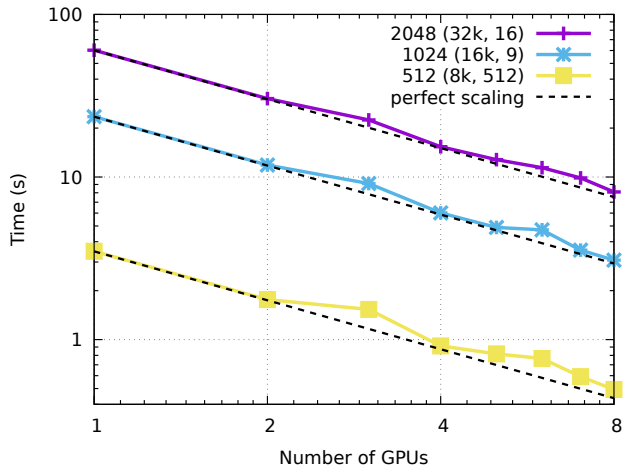
- When plotting strong/weak scaling performance, do not forget about the "ideal" line.
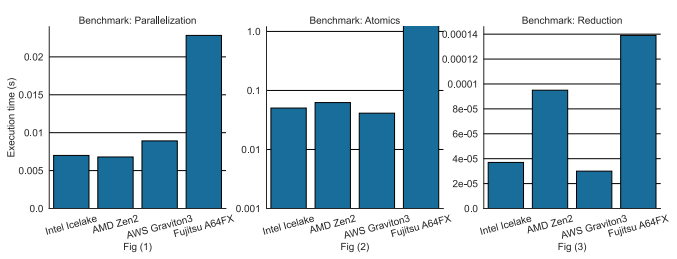
What not to do
Examples of bad plots (think why)